The field of algorithms is vast. Humans have been designing algorithms since antiquity, e.g. GCD algorithm. Of course, algorithms are the backbone of the current information age. Here are just a select few which have fascinated me because of their simplicity and cleverness.
Binary Search, Quick Sort & Quick Select
Given a list of items, sorting the list or searching for a given item, or selecting the minimum (or maximum) are ubiquitos programming problems. There are also multiple algorithms for each of those operations, each with their own advantages and disadvantages. Standard sorting algorithms are: Bubble Sort, Merge Sort etc. Nowadays, since there are standard library solutions to sorting, searching and selecting in all popular programming languages, programmers don't have to think about them so much. However, it helps to understand the technique behind the algorithms if you are dealing with a large data set. Binary search, Quick sort, and Quick select all use a similar, elegant technique and are also efficient algorithms.
Searching means you are given a sorted array and you have to find a particular element in it. Binary search algorithm uses a neat trick. Pick the middle element of the array, which then roughly divides the array into two halves. If you are lucky, and the middle element is what you are looking for, then stop there. Otherwise, now you have to search in just one half of the array, depending on whether the middle element is smaller or larger than the target you are searching for. Then whichever half you have to search on, run binary search on that half.
This way, the array to be searched is being halved at each stage. Hence, the time complexity is O(log n).
Sorting involves arranging all the elements of the array in order. Quick sort uses the same basic idea as Binary search. Each each step, pick a pivot element, swap elements so that left of pivot is smaller and right is larger. Now, recursively run Quick sort on both halves. Quick sort runs in O(n log n) average time but O(n2) worst case time.
Selection is the problem where you need to find the kth smallest (or largest) element in an unsorted array. Note that if the array is sorted, finding the kth smallest element is trivial. It means just looking up the kth index which takes constant time O(1). If the array is unsorted, Quick select algorithm uses the same technique as above. In the average case it takes O(n) time where as a naive algorithm using sorting would take O(nlog n). However, its worst case is O(n2).
1. Choose a pivot element from the array
2. Rearrange the array, such that elements smaller than the pivot are on the left, and greater ones are on the right
3. If pivot is in kth position, return the pivot element
4. If pivot's position is less than k, search for kth smallest in the left part
5. If pivot's position is greater than k, then search for (k - length of left part)th element in the right part
When you call up your bank's customer care, the call center agent asks you some questions to verify you are genuinely the account's owner. For example, they may ask the last 4 digits of your card number, your date of birth etc. By answering them correctly, you prove to the agent that you are indeed the person you are claiming to be. However, there is a problem in this scheme. Now, the agent also knows some details about you. It is possible that the agent may sell that data or even try to impersonate you and get undue access to your account. It would be ideal if you could prove to the agent that you are the genuine person without revealing any additional information in the process. Such a scheme is called Zero Knowledge Proof (ZKP). Let us look at the quintessential example:
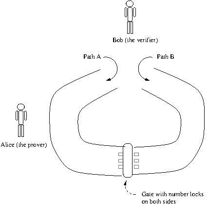
ZKP demo
There are two path A and B. Both lead to a gate. The gate has a number lock and can be opened from either side by entering a numeric pin. The pin is only known to select few. Alice knows the pin and Bob wants to verify that Alice does really know the pin.
Alice can simply tell the pin to Bob but then Bob would also get to know the pin. If Alice enters through one of the paths and opens the gate to let Bob come in and verify, then Bob would also get to enter the gateway, which is giving priviledged access to Bob. Hence, neither of these solutions are Zero knowledge.
The solution is: Alice enters through one of the paths A or B, then Bob picks A or B randomly and asks her to return via that path. If Bob asked for a different path than what Alice got in through, then she must enter the door, lock it back and come back up. Hence, proving that she knows the pin and in the process Bob learned nothing extra. To reduce the possibility of fluke, Bob can get Alice to do the same excersice multiple times. This is essentially the core or ZKP.
ZKP can be used to verify that a user knows the password, without revealing the password itself. It is also used in Blockchain to verify the ownership of a ledger entry. Here is how ZKP can be used to prove isomorphism of two graphs. Note that it follows the exact same scheme as above.
Two graphs G1 and G2 are called Isomorphic if they are same if we just rename the vertices appropriately. Let us say, someone (Alice) knows that two graphs G1 and G2 are isomorphic, i.e. G2 = π(G1). They want to convince another person (Bob) of this fact, but without revealing the mapping π of the vertices. Here is the algorithm:
1. Prover (Alice) picks a random permutation of vertices σ and creates a new graph H = σ(G₁) i.e., H is a shuffled version of G₁
2. Prover (Alice) sends H to the Verifier (Bob)
3. Verifier flips a coin and randomly chooses a bit b which can be either 0 or 1.
4. If b is 0, Verifier asks Prover to show that H is isomorphic to G₁. If b is 1, Verifier asks to show that H is isomorphic to G₂
5. Prover responds with the proof like this:
   If verifier asked for G1, send σ.
   Otherise, if prover asked for G2, send σ ∘ π⁻¹ (composition of σ with inverse of known isomorphism π)
6. Verifier checks whether applying the returned permutation to G₁ or G₂ gives H.
The above steps, never reveals the mapping π to the verifier. Instead, prover only reveals the mapping to a random graph. Hence making it a ZKP. As before, the verifier can ask the prover to do it multiple times to rule out a match by fluke.
Let us say, you are given an array. And you have to find a list of consecutive elements in the array whose sum is maximum. This is called the maximum subarray sum problem. Note that, if all the numbers are positive, then the maximum subarray is just the entire array. Similarly, if all numbers are negative, then it is just the largest value element in the array. So, maximum subarray problem is only interesting if the array contains a mix of positive and negative numbers. Only then, the cumulative sum of subarrays keeps increasing and decreasing as you move through the indices across the array.
Interestingly, maximum subarray sum problem occurs as a sub-problem within many larger problems. Kadane's algorithm is a single pass O(n) algorithm to solve this problem. It is deceptively simple.
# max_with_elem: maximum of all subarrays ending at the current index
# overall_max: overall maximum subarray found so far
# Within the loop, max_with_elem is updated as follows:
# either start a new subarray from the current element or extend the previous subarray
def max_subarray_sum(list)
  max_with_elem = 0
  overall_max = -Float::INFINITY
  list.each { |elem|
    max_with_elem = [elem, max_with_elem + elem].max
    overall_max = [overall_max, max_with_elem].max
  }
  return overall_max
end
Let us take an example: A cricketer has scored the following runs in last 10 innings: 43, 12, 54, 43, 62, 51, 70, 73, 1, 62. What is the longest streak where he scored above average?
# Last 10 matches
scores = [43, 12, 54, 43, 62, 51, 70, 73, 1, 62]
total = scores.sum
average = scores.sum / scores.size.to_f
# Let us assign above average score = 1, below average score = -1
markers = scores.map { |s| s >= average ? 1 : -1 } # the resulting array: [-1, -1, 1, -1, 1, 1, 1, 1, -1, 1]
# count the longest subarrays with 1s
max_subarray_sum(markers) # the result will be 4, which is the longest streak of 1s in the markers array
It is possible to enhance the above algorithm to also record the start and end indices of the selected subarray.
Given a string, it transforms the string to a version which has repeated characters together. With repeated characters, the string can then be compressed easily using Run length Encoding or Huffman encoding. Most importantly, the transformation is reversible, so it is easy to get the original string back after decompression. For example, given the string canada, first we need to add $ to the end of the string (any character can be used but it should be lexicographically smallest - i.e. a char that always comes first while sorting). canada -> canada$. Then calculate BW transform of the string which comes out to adnc$aa. Note that it has repeated characters aa and hence can be compressed. Reverse BW transform of adnc$aa then comes out to canada$.
Here is the BWT algorithm: 1. Generate all rotations of the string
How do you select k random items from a stream i.e. a list of unknown, and possibly large size without storing the whole list? Reservoir Sampling algorithm is a deceptively simple algorithm that works in O(k) space and guarantees that the final selection is a random permutation of the whole stream.
Here is the algorithm in its full glory:
1. Select the first k elements.
2. When a new ith element is received, select it with probability k/i
3. If the element is selected, replace a random element in the reservoir with the newly selected element.
The algorithm maintains an array of k elements and keep filling the array or replacing the elements in the array as new elements are received on the stream.
This algorithm finds use in sampling few lines from a large log file or records from a large data set, escpecially when we don't know the size of the data set. Note that, if we know the size of the stream in advance, say it is N, then selecting k out of N elements is straightforward since it only requires randomly selecting k indices.
Let us say you have a list of cities - Delhi, Jaipur, Kolkata, Indore and Mumbai. You also have a list of addresses of users. You have to classify each address into one of these cities. However, the addresses were sloppily written and have spelling mistakes in the city field. e.g. some address have city written as Dehli, Kalkatta etc. but it should still go into the right intended bucket of Delhi and Kolkata.
To solve this problem, you may want to calculate the distance of the filled city string from each city bucket. Then if the distance is small enough, classify it with that bucket. Here, distance could be defined as number of characters you have to edit, insert or delete to convert one string into another. For example, distance between Kalkatta and Kolkata is 2 since you can change a to o and delete one t. Since the distance is only 2, it may be considered close enough. This kind of distance between two strings is called Levenshtein distance. Here is the algorithm to calculate the Levenshtein distance between two given strings:
def ldist(str1, str2)
  if str1.size == 0
    str2.size
  elsif str2.size == 0
    str1.size
  elsif str1[0] == str2[0]
    ldist(str1[1..-1], str2[1..-1])
  else
   1 + [ldist(str1[1..-1], str2), ldist(str1, str2[1..-1]), ldist(str1[1..-1], str2[1..-1])].min
  end
end
It is a recursive algorithm. The same algorithm could also be written without iteratively using a matrix. The time complexity is O(m*n). Some optimizations are also available if edit sequence is not needed or if approximate answer is acceptable (see here).
Knuth's dancing links technique
In a circular doubly linked list, it is a simple operation to remove a node out of the list and also to restore it back to the list in the same position. Here is a doubly linked list:
will restore x's position in the list, assuming that x.right and x.left have been left unmodified.
Amazingly, it works in all cases. Even if the list has just one node. This simple observation is called Dancing links technique. This technique can be used to make searching easy in some cases where you want something to be removed temporarily and restored back later on if needed. Knuth presented a solution of set cover problem called Algorithm X which uses this technique called DLX. Algorithm X solves the exact cover problem (Given a set and list of subsets S, identify the set of subsets S* which cover the set where all subsets in S* are mutually disjoint). Many optimization problems like Sudoku, 8-queens problem are exact cover problem. They are typically solved using backtracking.
But Dancing links is a generic idea which can be used in other algorithms as well.
String matching algos
Finding a substring within a string is one of the most common action programmers have to do. You are given a large text and a small string, called pattern. The problem is to find out whether the pattern string occurs anywhere in the text.
Rabin-Karp algorithm finds the pattern using hashing. Iteratively, calculate hash of the sub-strings within the text and compare with hash of the pattern. A rolling hash is used so that hash of next substring can be calculated quickly. False positives because of hash collision can occur. So after a match is found, character by character comparision is performed. Average case is linear time O(m+n) but worse case is O(mn). It is used to detect plagarism in a document and is also used in data de-duplication.
Boyer Moore algorithm (ref) is used in GNU/Linux's all too familiar grep command. Pattern is checked against a part of the text, then slided forward and checked again. The main innvovations are: the pattern is checked starting with the end of the pattern. In case of a failed match, the pattern is shifted forward not just by one but several characters based on two rules: bad character rule and good suffix rule. Pattern is pre-processed and look up tables for applying the two rules are prepared before the search starts. Each rule give a number of characters by which pattern can be shifted. Maximum of these two is then taken as the shift value.
Sequitur algorithm or Nevill-Manning–Witten algorithm
In Formal language theory, a Context Free Grammar (CFG) is a formal grammar to describe patterns of strings (also called languages). Here is an example CFG:
S -> aSa
S -> bSb
S -> a | b
To generate a string that follows this grammar, start with symbol S. Then replace S by aSa (as per rule 1). Then replace the middle S by b (per rule 4) which then gives the string aba. Following similar patterns, we can see that strings produced by this grammar are like: a, b, aba, bbabb, etc. Basically, the grammar describes all palindromes using a and b. In other words, this grammar succintly describes the set of all palindromes using a and b. By the way, all programming languages are also CFG.
Now, lets reverse the problem. Given a string, can we construct a CFG for this string. Since, a CFG may be more compact than the actual string, hence may considered a compressed form of the string. Amazingly, the Sequitur algorithm does just that. Given a string, it produces a CFG which is without recursion and is often very compact.
The algorithm applies 2 Rules. Digram rule is when 2 characters which occur more than once in the sequence, is replaced by a rule in the grammar. Utility rule says if a grammar rule is used only once, remove the rule and replace the grammar rule using it by the string itself. Using these two straightforward rules, with a single pass over the string, the grammar is created.
Duff's device is an offbeat technique of loop unrolling to reduce the time taken by a loop in C programming language. It reduces the readability of the code and also violates the DRY (don't repeat yourself) principle of coding. But, it may give a speed boost when no other optimizations are possible. It is also fascinating to look at.
Each iteration of for loop checks the condition. If the condition check code is complex, it may slow down the loop. Loop unrolling tries to prevent that by duplicating the loop body several times so that the condition check happens lesser number of times. Note that, modern compilers do loop unrolling automatically. So this kind of tricks are not needed unless in extreme situations.
Here is a for loop which fills an array mylist with random numbers
  for(i=0; i < size; i++){
    mylist[i] = rand();
  }
Here is the same loop but unrolled. Note that each loop has the body repeated 8 times. Hence, the condition checks happen 1/8th number of times compared to the for loop above.
  int rounds = size / 8;
  int i = 0;
  switch (size % 8) {
  case 0:
      while (rounds-- > 0) {
          mylist[i++] = rand();

      case 7: mylist[i++] = rand();
      case 6: mylist[i++] = rand();
      case 5: mylist[i++] = rand();
      case 4: mylist[i++] = rand();
      case 3: mylist[i++] = rand();
      case 2: mylist[i++] = rand();
      case 1: mylist[i++] = rand();
      };
  }
This technique takes advantage of the C feature that if you don't put a break after a case, it will go on executing all the following cases. In C, each case is just a label to which code makes a jump (old fashioned GOTO). A while loop is also just a label to which jump is made from the end of the block. Hence, the switch and while statements can be interleaved together in this weird way!
Secretary Problem
An administrator wants to hire a secretary. The interview process has been set up in this way: the candidates will show up before the hiring administrator one after another. The administrator can either hire a candidate on the spot or reject her and call the next candidate. A candidate once rejected cannot be called back. Now the problem is: if the administrator wants to hire the best candidate overall, what should be their strategy?
The same problem occurs in many situations. From social situations like screening candidates for dating or marriage, to technical situations like allocating the best server of a CDN to users.
A completely naive solution would be to hire someone at random. But then the probability that she is the best candidate of the whole lineup is only 1/N. A better alternative would be to keep screening candidates till we get someone who is best of the lot seen so far. But then, there is a risk that we decided too soon. Perhaps, screening few more would have resulted in a better candidate. A generic form of this strategy is stated like this: screen first r candidates but reject them. After that, select the first candidate who is the best seen so far including the first r who were rejected.
Notice that r=0 was our naive strategy described above.
There is an elegant proof that if we pick r = N/e then the probability that we actually get the best candidate is 1/e ~ 36.8% which is impressive!
The two important things to keep in mind for this algorithm to work is: Number of candidates should be known in advance. Secondly, candidates themselves should not be aware of the strategy. Since the first r are going to be rejected, no one would want to go very early.